GRU Introduction
Gated recurrent units (GRUs) are a gating mechanism in recurrent neural networks, introduced in 2014 by Kyunghyun Cho et al. GRU is a very effective variant of LSTM network, which is simpler and more effective than the structure of LSTM network. It combines the forget gate and the input gate into a single "update gate". It also combines cell state and hidden state, and makes some other changes. The resulting model is simpler than the standard LSTM model. Detailed description below.
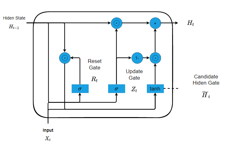
The first thing we need to introduce are the reset gate and the update gate. We engineer them to be vectors with entries in (0,1) such that we can perform convex combinations. For instance, a reset gate would allow us to control how much of the previous state we might still want to remember. Likewise, an update gate would allow us to control how much of the new state is just a copy of the old state. Given the input of the current time step and the hidden state of the previous time step. The outputs of two gates are given by two fully-connected layers with a sigmoid activation function.
Mathematically, for a given time step \(t\), suppose that the input is a minibatch \(\mathbf{X}_{t} \in \mathbb{R}^{n \times d}\) (number of examples: \(n\), number of inputs: \(d\) ) and the hidden state of the previous time step is \(\mathbf{H}_{t-1} \in \mathbb{R}^{n \times h}\) (number of hidden units: \(h\) ). Then, the reset gate \(\mathbf{R}_{t} \in \mathbb{R}^{n \times h}\) and update gate \(\mathbf{Z}_{t} \in \mathbb{R}^{n \times h}\) are computed as follows: \[ \begin{aligned} \mathbf{R}_{t} &=\sigma\left(\mathbf{X}_{t} \mathbf{W}_{x r}+\mathbf{H}_{t-1} \mathbf{W}_{h r}+\mathbf{b}_{r}\right) \\ \mathbf{Z}_{t} &=\sigma\left(\mathbf{X}_{t} \mathbf{W}_{x z}+\mathbf{H}_{t-1} \mathbf{W}_{h z}+\mathbf{b}_{z}\right) \end{aligned} \] where \(\mathbf{W}_{x r}, \mathbf{W}_{x z} \in \mathbb{R}^{d \times h}\) and \(\mathbf{W}_{h r}, \mathbf{W}_{h z} \in \mathbb{R}^{h \times h}\) are weight parameters and \(\mathbf{b}_{r}, \mathbf{b}_{z} \in \mathbb{R}^{1 \times h}\) are biases. And we use sigmoid function to transform input values to the interval \((0,1)\) \[ \sigma(x) = \frac{e^x}{1+e^{x}} \] Next, let us integrate the reset gate \(\mathbf{R}_{t}\) with the regular latent state updating mechanism in (8.4.5). It leads to the following candidate hidden state \(\tilde{\mathbf{H}}_{t} \in \mathbb{R}^{n \times h}\) at time step \(t\) : \[ \tilde{\mathbf{H}}_{t}=\tanh \left(\mathbf{X}_{t} \mathbf{W}_{x h}+\left(\mathbf{R}_{t} \odot \mathbf{H}_{t-1}\right) \mathbf{W}_{h h}+\mathbf{b}_{h}\right), \] where \(\mathbf{W}_{x h} \in \mathbb{R}^{d \times h}\) and \(\mathbf{W}_{h h} \in \mathbb{R}^{h \times h}\) are weight parameters, \(\mathbf{b}_{h} \in \mathbb{R}^{1 \times h}\) is the bias, and the symbol \(\odot\) is the Hadamard (elementwise) product operator. Here we use a nonlinearity in the form of tanh to ensure that the values in the candidate hidden state remain in the interval \((-1,1)\). \[ tanh(x) = \frac{sin(x)}{cos(x)} = \frac{e^x-e^{-x}}{e^x+x^{-x}} \] Finally, we need to incorporate the effect of the update gate \(\mathbf{Z}_{t}\). This determines the extent to which the new hidden state \(\mathbf{H}_{t} \in \mathbb{R}^{n \times h}\) is just the old state \(\mathbf{H}_{t-1}\) and by how much the new candidate state \(\tilde{\mathbf{H}}_{t}\) is used. The update gate \(\mathbf{Z}_{t}\) can be used for this purpose, simply by taking elementwise convex combinations between both \(\mathbf{H}_{t-1}\) and \(\tilde{\mathbf{H}}_{t}\). This leads to the final update equation for the GRU: \[ \mathbf{H}_{t}=\mathbf{Z}_{t} \odot \mathbf{H}_{t-1}+\left(1-\mathbf{Z}_{t}\right) \odot \tilde{\mathbf{H}}_{t} \] Whenever the update gate \(\mathbf{Z}_{t}\) is close to 1 , we simply retain the old state. In this case the information from \(\mathbf{X}_{t}\) is essentially ignored, effectively skipping time step \(t\) in the dependency chain. In contrast, whenever \(\mathbf{Z}_{t}\) is close to 0 , the new latent state \(\mathbf{H}_{t}\) approaches the candidate latent state \(\tilde{\mathbf{H}}_{t}\). These designs can help us cope with the vanishing gradient problem in RNNs and better capture dependencies for sequences with large time step distances. For instance, if the update gate has been close to 1 for all the time steps of an entire subsequence, the old hidden state at the time step of its beginning will be easily retained and passed to its end, regardless of the length of the subsequence.
